Coulomb Wave Funcitons

As a part of my master's thesis I had to make a numerical implementation of the Coulomb wave functions. The Coulomb wave equation for a charged particle with arbitrary angular momentum and charge is given by

\[ \nabla^2\psi +\left( k^2-\frac{2\mu}{\hbar^2}V(r)\right)\psi = 0, \]

where \(\mu\) is the reduced mass of the system. The radial wave function \(u(r)\) satisfies the following differential equation

\[ \frac{\text{d}^2 u_\ell}{\text{d}r^2}+\left( k^2-\frac{\ell(\ell+1)}{r^2}-\frac{2\mu}{\hbar^2}\frac{Ze^2}{r}\right)u_\ell=0, \]

where \(Z\) is the product of the charges. Two independent solutions can be found to this equation – these are called the regular and irregular Coulomb wave functions denoted \(F_\ell(r)\) and \(G_\ell(r)\) respectively. The regular Coulomb wave function \(F_\ell(r)\) is a real function that vanishes at \(r=0\) and the behaviour of the function is described using a parameter \(\eta\) which describes how strongly the Coulomb interaction is

\[ \eta = \frac{Zmc\alpha }{\hbar k}, \]

where \(m\) is the mass of the particle, \(k\) is the wave number and \(\alpha\) is the fine structure constant. The solution to is given by

\[ F_\ell(\eta,kr) = C_\ell (\eta) (kr)^{\ell+1}\text{e}^{-ikr} {}_1 F_1(\ell+1-i\eta,2\ell+2,2ikr), \]

where \({}_1F_1(kr)\) is a confluent hypergeometric function and \(C_\ell(\eta)\) is a normalization constant given by

\[ C_\ell(\eta) = \frac{2^\ell \text{e}^{-\pi\eta/2}|\Gamma(\ell+1+i\eta)|}{(2\ell+1)!}, \]

where \(\Gamma\) is the gamma function. For numerical purposes, it is useful to use the integral representation of the regular Coulomb wave function

\[ F_\ell(\eta,\rho) = \frac{\rho^{\ell+1}2^\ell e^{i\rho-(\pi\eta/2)}}{|\Gamma(\ell+1+i\eta)|} \int_0^1 e^{-2i\rho t}t^{\ell+i\eta}(1-t)^{\ell-i\eta} \, \text{d}t. \]

This implementation will need the gamma function from SpecialFunctions.jl. First we define complex integration

using QuadGK, SpecialFunctions, Plots

function complex_quadrature(func,a,b)
    function real_func(x)
        return real(func(x))
    end
    function imag_func(x)
        imag(func(x))
    end
    real_integral = quadgk(real_func,a,b)
    imag_integral = quadgk(imag_func,a,b)
    return real_integral1 + 1im*imag_integral1
end

And we can now define the regular and irregular Coulomb wave functions

function regular_coulomb(ℓ,η,ρ)
    First = ρ^(ℓ+1)*2^ℓ*exp(1im*ρ-(π*η/2))/(abs(gamma(ℓ+1+1im*η)))
    Integral_value = complex_quadrature(t -> exp(-2*1im.*ρ*t)*t^(ℓ+1im*η)*(1-t)^(ℓ-1im*η),0,1)
    return First.*Integral_value
end

function C(ℓ,η)
    return 2^ℓ*exp(-π*η/2)*(abs(gamma(ℓ+1+1im*η))/(factorial(2*ℓ+1)))
end

function irregular_coulomb(ℓ,η,ρ)
    First = exp(-1im*ρ)*ρ^(-ℓ)/(factorial(2*ℓ+1)*C(ℓ,η))
    Integral_value = complex_quadrature(t -> exp(-t)*t^(-ℓ-1im*η)*(t+2*1im*ρ)^(ℓ+1im*η),0.01,1e4)
    return First.*Integral_value
end

Examples

To test the implementation consider the following examples

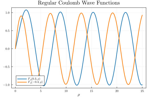
x = range(0,25,1000)
plot(x,regular_Coulomb.(0,0.3,x), label=L"F_0(0.3,ρ)")
plot!(x,regular_Coulomb.(0,-0.3,x), label=L"F_0(-0.3,ρ)")
xlabel!(L"ρ")
title!("Regular Coulomb Wave Functions")

Which will show the following

Use a similar approach to plot the regular Coulomb functions for different a \(\ell\)

x = range(0,25,1000)
plot(x,regular_Coulomb.(1e-5,5,x), label=L"F_0(5,ρ)")
plot!(x,regular_Coulomb.(1,5,x), label=L"F_1(5,ρ)")
plot!(x,regular_Coulomb.(2,5,x), label=L"F_2(5,ρ)")
plot!(x,regular_Coulomb.(3,5,x), label=L"F_3(5,ρ)")
title!("Regular Coulomb Wave Functions")
xlabel!(L"ρ")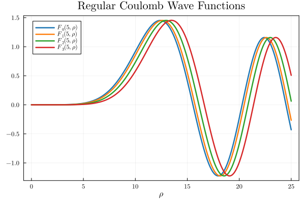

Solving non-linear partial differential equation numerically \(u_{xx}+u_{yy}=\mathrm{e}^{u}\)

This is a part of my answer on the Computational Science StackExchange to the differential equation

\[u_{xx}+u_{yy}=\mathrm{e}^{u}\]

with the following boundary conditions:

\[u(0,y)=a, \quad u_x(0,y) = b\] \[u(x,0)=c, \quad u_y(x,0) = d\]

Solution

Use something like MethodOfLines.jl to solve your problem. Modify the following example, something like this

using ModelingToolkit, MethodOfLines, DomainSets, NonlinearSolve

@parameters x y
@variables u(..)

Dx = Differential(x)
Dy = Differential(y)
Dxx = Differential(x)^2
Dyy = Differential(y)^2

eq = Dxx(u(x, y)) + Dyy(u(x, y)) ~ exp(u(x,y))

a = 5.2
b = 4.3
c = 3.5
d = 2.2

bcs = [u(0, y) ~ a,
       u(x, 0) ~ c,
       Dx(u(0, y)) ~ b,
       Dy(u(x, 0)) ~ d]


domains = [x ∈ Interval(0.0, 1.0),
           y ∈ Interval(0.0, 1.0)]

@named pdesys = PDESystem([eq], bcs, domains, [x, y], [u(x, y)])

dx = 0.1
dy = 0.1

discretization = MOLFiniteDifference([x => dx, y => dy], nothing, approx_order=2)

prob = discretize(pdesys, discretization)
sol = NonlinearSolve.solve(prob, NewtonRaphson())

u_sol = sol[u(x, y)]

using Plots

heatmap(sol[x], sol[y], u_sol, xlabel="x", ylabel="y",
        title="Solution")
		
savefig(joinpath(@OUTPUT, "heat.png"))

Where I've plugged in some random boundary conditions.

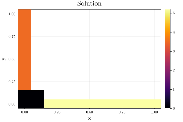
Where the white space is due to the non-linearity of the differential equation.

Optimal quadrature rule for heavy tail measure

This is my solution to the following question:

I'm looking for a well-thought quadrature rule for this measure \(d\mu(t)=\frac{dt}{t^s}\) for \(s\in(0,1)\), the underlying motivation is to compute this integral

\[ \lambda^{s-1}=\frac{1}{\Gamma(1-s)}\int_{0}^{\infty} e^{-t\lambda}\frac{dt}{t^s} \]

with \(\lambda > 0\), see this reference, Page 5, equation (5), https://arxiv.org/abs/1808.05159. So I'm looking for a way of dealing with the singularity at \(t=0\) as well as the limit to \(\infty\). Observe that

\[ \int_{T}^\infty \frac{dt}{t^s} = \infty \]

I was using the QuadGK.jl package and it is working just fine

λ = 2; s = 0.8
λs = λ^(s-1)

f(t) = exp(-λ*t)/t^s/gamma(1-s)
res, err = quadgk(f,0,Inf)

The predicted error and the real error is the same order of magnitude. However, when using the package for another formula

\[ \lambda^s = \frac{1}{\Gamma(-s)}\int_0^\infty (e^{-t\lambda}-1)\frac{dt}{t^{1+s}} \]

same reference as before. I again do the quadrature

λs = λ^s
g(t) = (exp(-λ*t)-1)/t^(1+s)/gamma(-s)
res, err = quadgk(g,0,Inf)

it works just fine, but this time the real error is of order 1e-3 while the predicted error is around 1e-8. And if I put a positive matrix instead of a scalar

A = # some positive definite matrix
h(t) = (exp(-A.*t)-I)/t^(1+s)/gamma(-s)
res, err = quadgk(h,0,Inf)

I get an ERROR: DomainError with 0.5: integrand produced NaN in the interval (0.0, 1.0), and, to my understanding, quadgk does not evaluate the function at \(0\) as per the documentation https://juliamath.github.io/QuadGK.jl/stable/. And if I write

res, err = quadgk(h,1e-50,Inf)

the integral blows up.

Solution

You can split the integral up such that you don't get the singularity at \(t=0\). Something like this

using QuadGK
using SpecialFunctions 

λ = 2.0; s = 0.8
λs = λ^(s-1)

f(t) = exp(-λ*t)/t^s/gamma(1-s)
@show res, err = quadgk(f,0,Inf)

λs = λ^s
g(t) = (exp(-λ*t)-1)/t^(1+s)/gamma(-s)
@show res, err = quadgk(g,0,Inf)

A = [2 -1 0; -1 2 -1; 0 -1 2] # some positive definite matrix
h(t) = (exp(-A.*t)-I)/t^(1+s)/gamma(-s)

singularity_integral, singularity_error = quadgk(h, 1e-10, 1e-5)
regular_integral, regular_error = quadgk(h, 1e-5, Inf)
@show result = singularity_integral + regular_integral
@show error = singularity_error + regular_error

which will print

(res, err) = quadgk(f, 0, Inf) = (0.8705505365052336, 1.2164780075652479e-8)
(res, err) = quadgk(g, 0, Inf) = (1.7402976255082268, 2.515036776166618e-8)
result = singularity_integral + regular_integral = [1.6837899364901885 -0.7050512093960599 -0.03988519645256732; -0.7050512093960599 1.6439047399317526 -0.7050512098966073; -0.03988519645256732 -0.7050512098966073 1.683789936502625]
error = singularity_error + regular_error = 3.822238569033589e-8

Alternatively, you can also look into something like [Cauchy principal values][https://en.wikipedia.org/wiki/Cauchyprincipalvalue] and [this example][https://juliamath.github.io/QuadGK.jl/stable/quadgk-examples/#Cauchy-principal-values]

–Edit: update to new information–

I'm afraid I can't reproduce the same error. When I run your code (I've added using LinearAlgebra for [diagm][https://docs.julialang.org/en/v1/stdlib/LinearAlgebra/#LinearAlgebra.diagm]) I get

res2 = [15.354655632950173 -6.419790221101635 -0.3665284746983265; -6.419790221101635 14.988127158828647 -6.4197902215468154; -0.3665284746983265 -6.4197902215468154 15.354655632887033]
norm(res2 + As) / norm(As) = 0.018647374162762107
norm(res1 + As) / norm(As) = 0.01864737561229984
norm(res1 - res2) = 4.9872522079524005e-8
4.9872522079524005e-8